[study] Statistical Thinnking

skim through widely known hypothesis tests, regressions, and sampling methods

Why statistics?

⭐ Reason 1. Project decision-making requires reasons based on data and numbers

⭐ Reason 2. Statistical thinking makes data easier to handle and more approachable.

T-test

T-test is a statistical test commonly used to determine whether there is a significant difference between the means of two groups.

The main criteria of this method is standard deviation.($\sigma$)

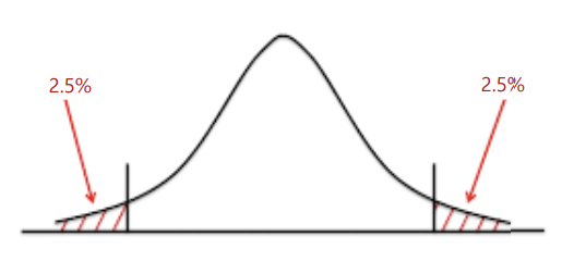
The null hypothesis and alternative hypothesis of t-test are the following:

$H_0 : \overline{X_a} = \overline{X_b}$
$H_1 : \overline{X_a} \ne \overline{X_b}$

If a t-value $\frac{\overline{X_a} = \overline{X_b}}{s/\sqrt n}$ is greater than a critical value, support the null hypothesis.
If a t-value is lesser than a critical value, reject the null hypothesis.

Degrees of Freedom

Degrees of freedom (df) indicates the number of values in a dataset that are free to vary.

The greater the degrees of freedom, the more accurate and precise a statistical analysis will be. (It can be used as standard normal distribution.)

In a t-test, the degrees of freedom is equal to the number of observations $n$ in the sample minus the number of parameters estimated from the sample.

One sample T-test

One sample T-test is used to test a single sample.
It is used to compare mean of a group to a certain $mu$ value.

from scipy import stats

t_stat, p_value = stats.ttest_1samp(series, mu)
print("t-statistics : {}, p-value : {}".format(t_stat, p_value))

t-statistics : -0.22787277117478616, p-value : 0.8202104280464514

since a p-value is greater than 0.05, the null hypothesis cannot be rejected.

Two sample T-test

Two sample T-test is used to compare distinct two samples.

from scipy import stats

t_stat, p_value = stats.ttest_ind(series1, series2,
                                  equal_var=True, alternative="two-sided")
print("t-statistics : {}, p-value : {}".format(t_stat, p_value))

t-statistics : -2.4809509135259113, p-value : 0.01392832955482604

since a p-value is lesser than 0.05, reject the null hypothesis

Thus, there is a significant difference between the mean value of two groups.

ANOVA

ANOVA (Analysis of Variance) tests the equality of means of two or more groups.

One-way ANOVA

One-way ANOVA compares the mean of two or more groups on a single dependent variable.

F-value

ANOVA method uses the F-distribution and the F-value to determine if the difference between the means of the groups is statistically significant.

The F-value is a measure of the ratio of variance between the means of different groups to the variance within the groups. It is used in ANOVA to determine whether there is a significant difference between the means of two or more groups.

The F-value is calculated by dividing the variance between the means of the groups by the variance within the groups. If the F-value is large, it suggests that the means of the groups are far apart, indicating a significant difference between the groups.

import statsmodels.api as sm
from statsmodels.formula.api import ols
from statsmodels.stats.anova import anova_lm

F, p = stats.f_oneway(series1, series2, series3)
print( 'F-Ratio: {}'.format(F)
    , 'p-value:{}'.format(p)
     , sep = '\n')

F-Ratio: 16.421131793497903, p-value:1.707725937052553e-07

since a F-value is greater than the critical value, reject the null hypothesis and at least one of the means of three series is different.

Two-way ANOVA

Two-way ANOVA compares the means of two or more groups on two different dependent variables.

model = ols('series3 ~ C(series1) + C(series2) + C(series3):C(series2)', data=cold_medicine).fit()
anova_table = sm.stats.anova_lm(model, typ=2)
anova_table

If all two independent variables and interaction effect have significant importance (F-value > critical value), all three variable needs post-testing. (Bonferroni / Sheffe / Turkey …)

Regression

Regression analyzes the relationship between a dependent variable and one or more independent variables. It is used to make predictions about the value of the dependent variable based on the values of the independent variables.

Simple Regression

Simple linear regression models the relationship between a dependent variable and a single independent variable.

from sklearn.linear_model import LinearRegression
import statsmodels.formula.api

# Generate Data
x = np.linspace(0,100,201)
e = 50 * np.random.randn(201)
y = [2*x[i] + e[i]  for i in range(201)]
reg_ex = pd.DataFrame({"x":x, "y":y})

line_fitter = LinearRegression()
line_fitter.fit(reg_ex["x"].values.reshape(-1,1), reg_ex["y"])

plt.plot(reg_ex["x"], reg_ex["y"], 'o')
plt.plot(reg_ex["x"],line_fitter.predict(reg_ex["x"].values.reshape(-1,1)))
plt.show()

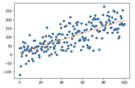
# predict y value from x input
line_fitter.predict([[75]])

array([149.83202999])

# coefficient and intercept
print(line_fitter.intercept_, line_fitter.coef_)

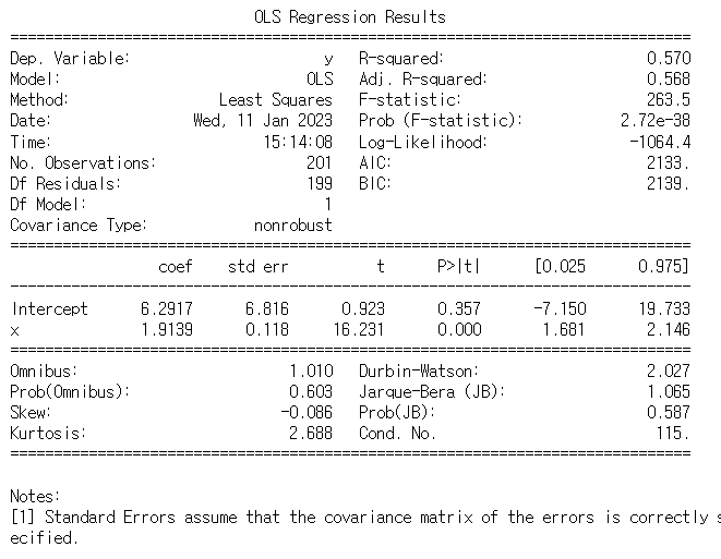
6.291671605500966 [1.91387145]

mod = statsmodels.formula.api.ols('y ~ x', data=reg_ex)
reg_result = mod.fit()
print(reg_result.summary())

Sampling

Sampling is the process of selecting a subset of individuals from a larger population to gather information about the population as a whole to make inferences about a population based on a smaller sample.

Rejection sampling

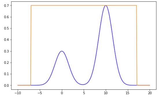
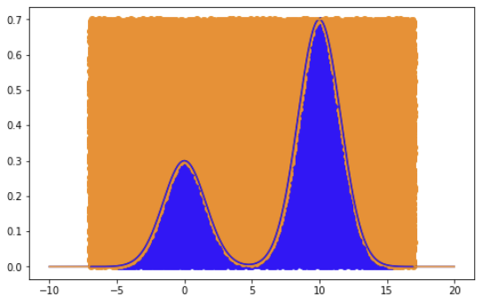
Rejection sampling generates random samples from a probability distribution that is difficult or impossible to sample from directly. The basic idea behind rejection sampling is to generate random samples from a known distribution that is easy to sample from and then reject samples that do not come from the target distribution.

import random
import numpy as np
import matplotlib.pyplot as plt
import matplotlib.mlab as mlab
from scipy.stats import uniform

x = np.linspace(-10, 20, 300)
plt.figure(figsize=(8, 5))
plt.plot(x, 0.3*np.exp(-0.2*(x**2)) + 0.7*np.exp(-0.2*(x-10)**2) , color='b')
plt.plot(x, 0.7/(1/24) *uniform.pdf(x, -7, 24), color='darkorange')
plt.show()

xdomain = [-7, 17]

def random_point_within_enveloping_region():
    """
    """
    x = random.uniform(xdomain[0], xdomain[1])
    y = random.uniform(0, 0.7)
    return (x,y)

#Number of sample points to sample
n = 10000

#Creating two arrays to capture accepted and rejected points
accepted = []
rejected = []

#Run this loop until we got required number of valid points
while len(accepted) < n:
 
    #Get random point
    x, y = random_point_within_enveloping_region()
 
    #If y is below blue curve then accept it
    if y < 0.3*np.exp(-0.2*(x**2)) + 0.7*np.exp(-0.2*(x-10)**2):
       accepted.append((x, y))
    #otherwise reject it.
    else:
       rejected.append((x, y))
    
#Plot the graph
x = np.linspace(-10, 20, 1000)
plt.figure(figsize=(8, 5))
plt.plot([x[0] for x in accepted], [x[1] for x in accepted] , 'ro', color='b') # Plot Accepted Points
plt.plot([x[0] for x in rejected], [x[1] for x in rejected] , 'ro', color='darkorange') # Plot Rejected Points
plt.plot(x, 0.3*np.exp(-0.2*(x**2)) + 0.7*np.exp(-0.2*(x-10)**2) , color='b')
plt.plot(x, 0.7/(1/24) *uniform.pdf(x, -7, 24), color='darkorange')
plt.show()

Reservoir sampling

Reservoir sampling randomly selects a fixed number of items from a large data stream or dataset without having to store all of the items in memory. It’s particularly useful when the dataset is too large to fit in memory and it’s not possible to process all the items in one pass.

The basic idea behind reservoir sampling is to maintain a “reservoir” of $r$ items, where $r$ is the number of items to be selected from the dataset, and to update the reservoir with new items as they are encountered. The algorithm works as follows:

import random
import sys

def reservoir_sampling(sampled_num, total_num):
    sample = []
    for i in range(0, total_num):
        if i < sampled_num:
            sample.append(i)
        else:
            r = random.randint(0, i)
            if r < sampled_num:
                sample[r] = i
    return sample